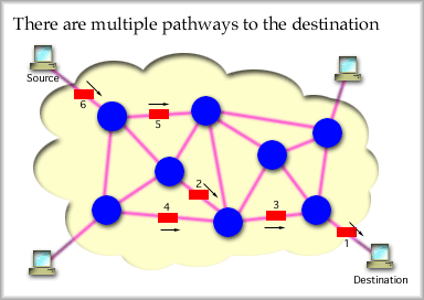
Read Chapter 9 and Chapter 19 as well as this lesson.  Then, complete the hw 9a.

Circuit Switching and Switching Networks
Switching is a process of connecting incoming signals to the proper outgoing channel.  Back when telephone operators handled all long distance calls, the operators manually interconnected the appropriate outgoing line with the incoming call.

Consider a mechanical switch, which directs a signal from an incoming line to the appropriate outgoing line.  You might be most familiar with a telephone switch, but there are also data switches.

Telephone Switch:  uses the phone number to determine which outgoing line to connect to.

Data Switch:  uses hardware address to decide which outgoing line to choose.

We can organize switching into two types:

Circuit Switching:  An incoming line is connected to an outgoing line and the lines are dedicated for use by this single connection.  In series, the connections build an end-to-end connection.  The Public Switched Telephone Network (PSTN) is a circuit switched network.

Packet Switching:  Individual packets, frames, or cells are accepted on one incoming line and sent out one outgoing line.  The lines are only used when the packet needs them, thus many connections can share the use of these lines.  The Internet is packet switched.

We will investigate packet switching in Lesson 9.  From this point, we'll concentrate on the public telephone network and how it uses circuit switching.

The Circuit Switched Telephone Network
All circuit switched connections, including the telephone system, set up a pathway between two end points that is dedicated for the duration of the "call".  Here, the word "call" can refer to both a voice call or a data call.  A dedicated circuit has some nice advantages.

• User gets exclusive use of this pathway.  It is not shared.
• Very little delay, once the call has been set up.
• User information rate can be guaranteed.
• Information arrives in the same order that it was sent in.

Of course there are some disadvantages as well.

• Very inefficient use of the media because of idle time.
• Other users trying to use the same circuit are blocked.  A good example is a busy telephone signal.
• Both ends have to establish identical connections to the network. An example here is modem speed.  Your modem has to accept data at the same rate that the data was sent at.
• Complete, end-to-end call set up is required before transmission of information can begin.

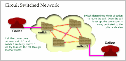
The above advantages and disadvantages are typical features of the PSTN, but also occur in circuit switched data networks. 

One feature of circuit switched connections is the need for complete call set up before any messages can be passed.  Sometimes, as you know, call setup fails  [43k sound clip]. After the call is set up users exchange full or half duplex messages (most likely full duplex) across the end-to-end circuit that is dedicated for their use.  Upon completion of the exchange, one user disconnects and the resources along the circuit are released becoming available for use by other users.

The following two graphics show two callers separated by three links.  Two switches perform circuit selection to route the call request through the network to the "callee."  If the callee accepts the call, a circuit is established.

The network layout:

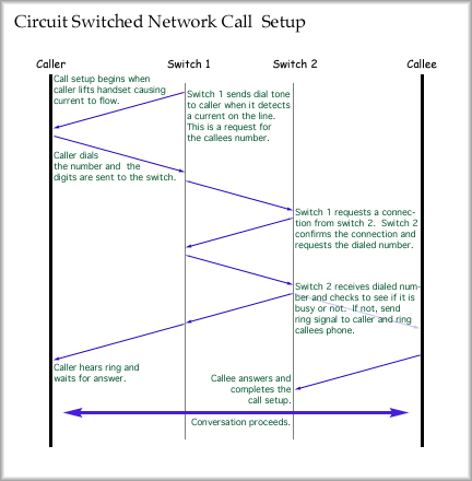
The call set up would proceed in this manner:

For the telephone system, circuit establishment would follow these steps, which agree with the small network and set up graphics above.

1. User picks up handset of telephone to make a call, electrical current begins to flow (an "off-hook" signal).  Current sensor in the telephone company's central office triggers the sending of dial tone to caller (nearly instantaneously).
2. Caller dials number and the switch, knowing the dialed number, selects the appropriate outgoing line by checking a database.  Then the switch requests a connection with the next switch along the chosen path, which we'll call Switch 2.
3. Switch 2 confirms the connection to Switch 1 and requests that the dialed number be sent.  Switch 1 sends the dialed number.
4. Switch 2, in this case, is the last switch before reaching the callee.  Switch 2 checks the callee's line to determine if it is in use.  If it is, a busy signal is returned to the caller.  If the callee's line is not in use, switch 2 will send a ring signal back through the network (which becomes a ringing tone on the callers line) and also rings the callee's phone. 
5. The end-to-end circuit is established if the callee picks up the phone.  From this point, there is a dedicated pathway through the network, a circuit from end to end.
6. Users communicate as necessary until one disconnects by hanging up.  The "on-hook" signal releases the connection to the switch.  The switch releases its connection to the other switch.  The release of each link cascades through the network all the way to the final link between the other user and the nearby switch.  This link is not released until the user hangs up.

Usually the user to network link is a permanent, dedicated connection that sits idle when not in use.  When the phone is "on-hook" there is no current flowing and the link idle.  It is, however, still dedicated for the use of the service subscriber.

The Telephone System
The PSTN, or public switched telephone network, has three main parts, the local loop, the central office and interoffice trunks.  In this section we will take a look at each of these.

The Central Office
The CO houses equipment to operate the telephone network.  The primary piece of equipment is the switch.  At the CO, an incoming call request must be directed to an appropriate outgoing line.  the address, a phone number in this case, provides the necessary information that a switch needs to consult a table and look up which outgoing line the call request should be routed to.  Outgoing lines between central offices are called trunks. 

Trunks
Between two central offices are groups of links.  There are not enough links to support calls by all users simultaneously, but that many links are not necessary.  It is extremely unlikely that every subscriber would pick up their phone and make calls simultaneously that need to be routed across the same set of trunks.  A single voice line between two central offices counts as one trunk.  Usually, there are many trunks between central offices and this bundle is called a trunk group.

By designing carefully, traffic engineers can provision the network with just enough trunks to meet demand.  This demand is not current demand, but the expected demand at the end of the "engineering interval".

For example, an engineer might specify that 32 trunks should be installed between two COs and that these should be sufficient to support the expected demand for service at the end of 5-years of use.

The engineering interval would include the design time, the installation time and the time in service.  At the end of this interval, the trunk group should meet the expected demand.

Unfortunately, it isn't always easy to specify the number of trunks to install.  Usually a T1 is used to provide service.  This means that trunks are installed in groups of 24.  In the example above, we could install one T1 with 24 trunk lines.  Twenty-four trunks is not very close to 32.  The engineer would expect the service on the trunk group to be overloaded, with customers getting (fast) busy signals if they couldn't be rerouted.

Our other choice is to install two T1 connections, or 48 trunks.  The traffic engineer has to make some decisions about which way to go here.  Perhaps an E1 could nearly meet the engineering interval.

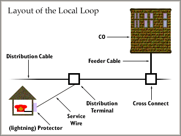
The "Local Loop"
The telephone system between the central office, or CO, and your home, including all the wires, poles, terminal boxes, manholes and other equipment is collectively called the "local loop" and sometimes "the last mile". 

The pair of copper cables that run from your home to the CO are solely dedicated to you.  Each subscriber has a unique pair of wires running all the way to the CO's switch.  This link is not shared, unless you have a party line, which is pretty rare these days.  The local loop is the most expensive part of the telephone system because of the amount of copper used and the installation time required to it.

Once your call reaches a telephone switch it has to compete for the limited number of outgoing lines, unless it immediately goes on to another local loop line.

The design of our current PSTN has been driven in the past by the need to support voice service.  Very little consideration was given to transmitting data across the network.

Now, we are trying to retrofit data systems so they can work over this network.  Digital Subscriber Line, or DSL, is one example of how the phone system can be reworked to support high data rates.

A migration of design goals is taking place now as data transmission becomes more and more important.  Your humble instructor predictions that data will become the primary engineering goal for the telephone network, that is if it hasn't already.

Packet Switching Principles
You studied in lesson 8 that circuit switching has some disadvantages.  The use of media is highly inefficient and blocking occurs.  Packet switching makes much more efficient use of the resources by allowing sharing to take place.

Packet switching operates in a simple manner.  A message is transferred, either in whole or in part, by hopping from node to node in the network.

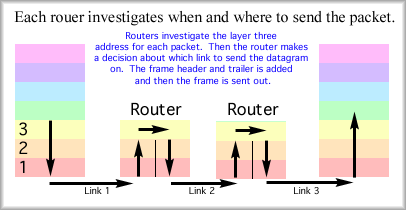
If the entire message is sent from one node to another node all at once, the transfer is called message switching.  This works with small messages, but with large messages, the information has to be broken up into smaller packets, also known as datagrams.  These operate at layer three of the OSI reference model.  The datagrams that comprise one message are not required to follow the same pathway through the network.  At each node in the network the datagrams are inspected and a decision about which direction to send them is made.  The decision process is called routing.

For routing to take place the datagrams must have destination addresses, and by convention, return addresses are also required.  The Internet uses IP addresses, with each machine on the Internet getting a unique address. 

With many packets running though the network along different pathways, the packets arrive out of order.  Layer four will fix that problem for us.  Layer three is just responsible for getting the packets from one end of the internetwork to the other.  Some of the other disadvantages are that processor power is required to rebuild messages, some delay occurs at each node as decisions are made on where to send the packet and headers get attached to each packet, not just once at the beginning of a message. 

Chopping up a message and delivering it is no easy task.  Each message has to have addressing information attached, error checking included and information on how to put the message back together properly.

Life of a datagram.
Lets take a look at the life of a single datagram.  This is true datagram service.  The datagrams in the network travel totally independently of each other. 

The datagram is born when a message is segmented into parts for transmission.  Layer four of the OSI model is responsible for doing this and for marking the segment with a number so it can be put back into order on the other end. 

Layer three receives the segment and tacks on a header.  The header includes the destination address and the return address.  Now called a packet, it is handed to layer two and a frame is built, such as for HDLC. 

Layer two, following the rules of access to the medium, passes the bits to layer one to be transmitted as signals over the physical link to the next node in the network.  The signals are received and converted to bits, layer two removes the info from the frame and hands that up to layer three.  This node, a router, looks at the address, makes a decision about which direction to send the datagram and then sends it out on the next link. 

To do this the packet travels down the OSI stack back through layer two and one.  The layer one signals are sent to the next node and the process is repeated.

Eventually, the datagram arrives at the end node, a workstation for example.  The signals are converted to bits, the bits are inspected by layer two as a frame and the frame header and trailers are removed.  The data field of the frame is handed up to layer three where the address information is checked.  Yes, this packet belongs here, so layer three strips off the layer three header and hands the data field up to layer four. 

Layer four, which we'll investigate in chapter 17, makes sure that all the packets have been received, reorders and rebuilds the original message.  That's as far as the datagram goes.  The message will likely work its way all the way up the OSI model to the application layer.

During its travels a datagram may encounter different local area network (LAN) protocols like Ethernet or Token Ring, various wide area networking (WAN) protocols like HDLC or Frame Relay, and different nodes like switches and routers.

Virtual Circuit Service
Virtual Circuit (VC) service draws benefits from both worlds, datagram packet switching and circuit switching.  A virtual circuit is simply a pre-chosen pathway through the network that all packets will follow.  Each packet is still inspected at intermediate nodes in the network to determine where they should be sent, but all packets follow the same path.  Packets following the same pathway will arrive in order.  This is the main advantage of a VC.  In addition, packets do not need to be numbered for reassembly at the destination.  X.25 is a packet switched virtual circuit service.  X.25 will appear later in this lesson.

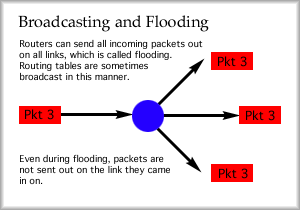
Both datagram and virtual circuit packet switching require decision making at the intermediate nodes, the routers.  Virtual Circuit will require "call setup", just like other circuit services, however.  During the call setup, each router will make a note of how particular packets should be routed.  Then, when packets from the VC comes in, they are routed in a consistent manner.

Routing
Routing is the decision making process of choosing an outbound link for a packet.  Routers usually have several links to choose from and the router uses IP address information stored in tables to make those decisions. 

Early networks started out by choosing links that would send packets across the fewest number of links, or hops.  The least number of hops was assumed to take the packet to the directly and quickly.  This isn't always so, however.  A few more hops at 20 times the capacity can be a significant improvement.

The concept of fewest hops is just one form of "least cost" routing.  Routing metrics (measurments) such as the number of hops, the capacity on a link, the links reliability and cost, may be important factors in the way packets are routed.  Least cost routing is something an administrator can configure on the router. 

One fairly simple process for making routing decisions is random routing .  Routers using this method of decision making balance the outgoing packets evenly between all links.  If needed, the network administrator can set the weighting of which links should get more or less of the packets.  An advantage is that packet addresses do not need to be investigated to implement this type of routing.  The assumption is that some other router will route the packets appropriately later on.

Broadcast routing is also fairly simple.  It is also sometimes called flooding.  Packets that arrive are sent out all other links.  Very important messages, like router updates (shared router table information) might be sent this way.

This might create a problem however, because it would be possible for these updates to continue running around the network forever.  For this purpose, a time-to-live (TTL) field is included in the packet.  One pass through a router is considered a single hop.  The TTL field will contain the maximum number of hops allowed.  As the packets move from router to router, the TTL field is decremented until it reaches zero.  Once there the packet is finally discarded.

Another simple process is fixed routing.  The router sends all packets received on a particular link out another particular link.  Actually, as mentioned by Stallings, we hope that routing is correct, simple, robust, stable, fair, optimal, and efficient. 

Adaptive routing , on the other hand, makes decisions on the fly based on the current situation.  This allows the router to adjust its routing decisions when links fail or when there is too much delay on an outgoing link.  As Stallings mentions in the text, most modern networks implement adaptive routing. 

Some of the routing protocols that you may encounter include RIP, OSPF, EIGRP, and BGP.

X.25 Packet Switching Protocol
X.25 is one example of a packet switching protocol that offers virtual circuit service.  It is a standard developed by the ITU-T for packet switched communications between your DTE and the packet switched network.

The X.25 standard is actually a suite of standards.  One for each of the first three layers of the OSI model. The important layers we'll look at are layers two and three. X.25 does not specify any standards at layers four or above.

• Layer 3 -- X.25 Packet Layer
• Layer 2 -- LAP-B (nearly identical to HDLC).
• Layer 1 -- X.21 Physical Interface

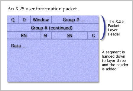
We won't investigate LAP-B frames because they are identical to HDLC.  The difference to note is that LAP-B only uses ABM mode for connections, the peer-to-peer connection method of HDLC.

The X.25 Packet Layer is responsible for establishing a virtual circuit and then for sending information frames to the destination.  To set up a virtual circuit, a call request is made.  Very similar to a circuit connection attempt for telephone "calls" a virtual circuit is setup one link at a time across the network.

After the call is setup, then sliding window protocol is used to manage the flow control.  Go-back-N is used as the error control.

After the data is exchanged, a clear request is sent and the virtual circuit is released.  This means that entries in the various routers' tables are cleared for that virtual circuit.

An X.25 packet format at layer three can be drawn as follows. 

• The Q bit is rarely used. 
• The D bit is used for ACK messages, either a 1 for a long distance ACK or a 0 for a local ACK.  The ACK is used during call setup. 
• Window is a term I use.  01 indicates that three bit sequence numbers are used (top three packet formats on pg. 286).  A 10 indicates that 7 bit sequence numbers are used (lower three packets on pg. 286).
• Group # is the virtual channel ID number.  Packets with this number can be routed by the router on the same link.  This field is 12 bits (it wraps around).
• RN is the receive number
• SN is the send number
• M is the more bit.  Data can be chopped up into smaller pieces and then put back together.  A 1 in the More field means that more pieces are still coming.  A zero means that this is the last piece.  Remember the pieces will arrive in order.
• C is the packet type and it is set to 0 only when user data is being sent.  Set this to 1 when sending control info or acknowledgments.

This packet will fit into a LAP-B frame at layer 2 and be sent as signals across the link from the DTE to the DCE.  Once the DCE accepts the frame, it may be sent out on virtual-circuit-switched packet networks of various protocols.

Note that there is no error checking in the layer three packet.  All the error checking occurs in the layer two LAP-B frame and maybe at higher layers.

X.25 was typically used to connect the user's DTE with a packet switching network's DCE.  IP is more common than X.25 today.

Used with permission of the Author; Copyright (C) Kevin A. Shaffer 1998 - 2018, all rights reserved.